Bitnets: Model weights in 1.58 bits

Running an LLM is expensive. A huge portion of that cost is attributed to the model weights. Typically, a large language model (LLM) has billions of parameters (or weights), and these weights take up some amount of storage in memory. Usually, each weight is represented as a 16-bit floating-point number (FP16 / BF16), and that is about 2 bytes per weight (or 16 bits). Now the math is easy: for every n billion parameters, you need 2n gigabytes of memory to load the model and run inference (e.g., a 2B model needs 4GB RAM).

Now this is not optimal, because to increase the overall intelligence of an LLM, it typically needs to have space to learn more information about the world, and this happens by increasing the parameter count. Frontier models (at the time of writing) are known to have multiple trillions of parameters (a good example of this is the newly dropped Kimi K3 open-weight model that contains 2.8 trillion parameters). Such heavy models make LLM inference costly in two phases: the prefill phase and the decode phase.

In the prefill phase, a model takes up your entire working prompt and does a bunch of calculations. This operation is bottlenecked by the compute a system has, so it's called a compute-bound operation. The prefill determines the TTFT, or the Time To First Token, metric. Prefill is the first order of operation during LLM inference. As a result, a larger model requires significantly more compute as it needs to perform a much bigger matrix multiplication for each input token. And the second phase is the decode phase, which determines the TPS, or the tokens per second, metric. This process involves rapidly reading the model weights from memory and performing matmul operations. This is run iteratively for every token that needs to be generated and is an extremely rapid process that's bottlenecked by how fast the weights can be read from the virtual memory. So, decode is called a memory-bandwidth-bound operation.

Post-training optimization

Typically, PTQ (post-training optimization) is a technique that is employed on LLMs to shrink their weights so that both of these operations (prefill and decode) can be sped up. Quantization is a process in which you shrink the precision of these weights. You can truncate them into various formats like FP8, INT8, or INT4. As a very rough example, if your weight is something like 3.141592 in FP16, then truncating the precision to INT8 makes the weight an integer and snaps it to a number within the INT8 range (-128 to 127).

The beauty of quantization is that the precision of these weights can be truncated to something like INT8 or INT4 for huge gains in memory/latency with a small compromise in intelligence. There is another technique called QAT (quantization-aware training) that lets you train an LLM to a smaller precision while quantizing the weights on the go at each iteration of training. And in practice, we are seeing huge gains in the efficiency of models that go through some quantization process. You can retain something around 95-99.99% capabilities of a model while shrinking it to half or even a fourth of its size.

1-Bit quantization

Now here's where bitnets come into play. Microsoft launched the official BitNet paper long ago with the idea of truncating weights into just 1-bit (either a 1 or a -1). This means a model is now binary. The results were quite fine, not too crazy, because the quality loss was not acceptable to a certain degree. Meaningful information seemed to be lost in the process of building a binary model of a class size similar to an FP16 model. Then, in the subsequent year, they launched another paper on building 1.58-Bit models. This essentially just introduces a third possible value for the weights, forming the set:

$$\{-1, 0, 1\}$$

And the strange 1.58 is just the representation of these 3 values by taking a logarithm of all possible values.

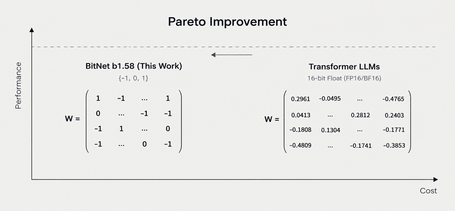
$$\log_2(2) = 1 \quad \{-1, 1\}$$$$\log_2(3) \approx 1.58 \quad \{-1, 0, 1\}$$

And what we noticed was that with the introduction of a third weight, we were able to reach model quality parity with FP16 using a model that was so much smaller, more efficient, and faster. The idea is that by representing weights as ternary values, we can perform computations much faster and with less memory overhead. Decode, especially, becomes so much faster because it's now faster to move these weights across memory to perform computations.

Mults become Adds

One more property that emerges when the model weights are ternary/binary is that matrix multiplication becomes a series of additions and subtractions - which are logically faster to compute at a hardware level compared to multiplication. How this works out is:

$$+1 \times x = x \qquad \text{add}$$$$-1 \times x = -x \qquad \text{subtract}$$$$0 \times x = 0 \qquad \text{skip}$$

Math behind the quantization

Simple steps are followed during training to ternarize a model's weights. Essentially:

1. Keep full-precision latent weights. They exist only during training.
2. Forward pass: quantize on the fly, compute with the ternary weights. The loss always sees the model as it will actually run.
3. Backward pass: the quantizer’s gradient is zero everywhere, so we employ a straight-through estimator that pretends it’s the identity and passes the gradient to the latents.
4. Latents accumulate tiny updates like votes; they cross the threshold, and the visible weight flips.
5. After training: throw the latents away. Ship ternary weights + one FP scale per matrix.

The "quantize on the fly" bit involves something known as absmean quantization. How this works is: you essentially take the absolute mean of all the weights, then round it to the nearest integer, and then clip it between -1 and 1. It looks something like this:

$$\widetilde{W} = \operatorname{RoundClip}\left(\frac{W}{\gamma + \epsilon}, -1, 1\right)$$$$\operatorname{RoundClip}(x, a, b) = \max\left(a, \min\left(b, \operatorname{round}(x)\right)\right)$$$$\gamma = \frac{1}{nm} \sum_{ij} \left|W_{ij}\right|$$

Results?

The ternary model with the addition of a 0 proved to be so much better than a binary model. This was because the 0 was able to do something called feature filtering. What this means in essence is that with the binary model previously ({-1, 1}), the activations were either entirely positive or negative, and there was no way for a neuron to act as though it were irrelevant for the specific feature. With the introduction of a third neutral value, 0, this changed the game entirely, making the model reach accuracy parity with its BF16 counterpart. We observed three things happening here:

1. Quality parity (at scale)

Perplexity (lower = better), BitNet vs LLaMA: at 700M it loses (12.87 vs 12.33); at 1.3B it's nearly even (11.29 vs 11.25); at 3B it wins (9.91 vs 10.04). Average task accuracy tells the same story: 44.3 vs 45.5 at 700M, 45.4 vs 46.2 at 1.3B, then 50.2 vs 49.7 at 3B.

This monotonic gap-closing is the most important pattern in the paper, more important than any single number. The intuition for why: larger models have more redundancy: many parameters encoding overlapping information. So they absorb the "damage" of coarse weights better. Each individual ternary weight is a terrible approximation; but with billions of them, and training that knows about the constraint, the ensemble recovers the function. One important thing to note is that below ~3B, parity does not hold. The claim is "at 3B and beyond," not "always."

2. Pareto improvement

At 3B: memory 2.22 GB vs 7.89 GB (3.55× less), latency 1.87 ms vs 5.07 ms (2.71× faster) with better perplexity. Then the flex: Microsoft trained a 3.9B BitNet that beats LLaMA-3B on every quality metric (PPL 9.62, avg accuracy 51.2) while still using less memory (2.38 GB) and less latency (2.11 ms) than the 3B FP16 model. That's the cleanest one-slide summary of "Pareto improvement": higher quality AND lower cost, simultaneously.

3. Gap grows with scale

The efficiency at 700M is modest, but we see real improvements only when the model size crosses the 3B threshold, and this is because smaller models have a lot more non-ternary layers where quantization collapses the whole layer. At sizes >= 3B, there is enough redundancy and space in the model such that ternarizing it actually produces a wide gap in efficiency, and it only grows larger with size. At 70B, decoding is 4.1× faster, and on two 80GB A100s, a batch size 11× larger fits, giving 8.9× throughput (2,977 vs 333 tokens/s). Energy: 71.4× lower arithmetic energy for the matmuls at 7nm.

---

Now these results also open up a lot more discussions around quite a few topics like mixture-of-experts models (ternary models can help fit all experts in memory because of their smaller sizes instead of being streamed from somewhere slower like a disk), running inference on edge devices, and customized hardware to run additions/subtractions at much higher speeds than traditional compute. As a proof of concept, we were able to take PrismML's Bonsai 27B model (at 1-bit) and run it on an iPhone, letting it do agentic actions.

And very recently (as of writing), PrismML also released Bonsai 2 - based on Qwen3.8 27B, with which they were able to retain a whopping 98% of the intelligence with a 9x smaller footprint. Our team at Conscious Engines is working a lot on foundational research at the intersection of ternary models and mixture of experts and is observing great results. All of this work is really exciting because it makes models smaller and faster and helps them dissolve into your workflows.